Building with lambda calculus
nthelt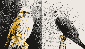
The Kestrel and the Kite. Photos by Jakub Hałun and Charles J. Sharp.

_young_adult.jpg)
One of us always lies, and one of us always tells the truth.
— The Kestrel
A lambda term is just a different way of writing a function. Like a normal function, a lambda term takes an input or inputs and returns something. The expression λa.a
reads from left to right as “takes a single input a, and returns a”. This is the simplest lambda term and it is equivalent to f(x) = x. Lambda terms can receive an input, for example x, from the right like so,
λa.a x.A function which takes an input and returns it unchanged, takes input x—what does that give us? x. So, the expression above can be reduced to simply x. You can also say that λa.a x
is equivalent to x. We’ll use a =>
symbol to indicate this reduction.
You can express all sorts of concepts in math and programming using just lambda terms. Let’s pick the coolest ones and build them from first principles.
A flock of functions #
Below are the standard named combinators, expressed as lambda terms. They’re fundamental building blocks which we can turn into compound concepts. Each has the name of a bird, and a mathematical object or two it’s equivalent to.
I = λa.a— Idiot: identity.M = λa.aa— Mockingbird: omega.K = λab.a— Kestrel: true, constant.KI = λab.b— Kite: false, zero.T = λab.ba— Thrush: not, switch.W = λab.abb— Warbler: ?C = λabc.acb— Cardinal: not.B = λabc.a(bc)— Bluebird: compose, multiply.V = λabc.cab— Vireo: pair, cons.S = λabc.ac(bc)— Starling: ?
For my full list of combinators expressed in lambda calculus, see Library of λ
The Kite for example takes two inputs and returns the first one unchanged. It can take term x
like so,
λab.a x => λb.x.We get this new term, which takes an input and throws it away, to instead return the term x. Now let’s feed that term another input y.
λb.x y => x.This is the same as if we fed both terms into the Kite at the same time.
λab.a x y => λb.x y => x.This process of feeding one input at a time is called Currying.
Booleans (Church-encoded) #
We can express boolean logic just with lambdas. Recall the classic programming pattern
if boolean then x else y.In the context of an if statement, the essence of a boolean is a function that selects between two arguments. Well, that’s exactly what we have in the Kestrel and the Kite. Let’s define our TRUE
and FALSE
combinators.
TRUE = K = λab.a— Picks the first of two inputs.FALSE = KI = λab.b— Picks the second of two inputs.
Take the expression BOOL x y, where BOOL
is either TRUE
or FALSE. If BOOL = TRUE, then this reduces to x. If BOOL = FALSE, then this reduces to y. This is what an if statement does.
We can also do boolean logic.
NOT = C = λabc.acb— Swaps the second and third inputs. i.e.
NOT TRUE = FALSESee if you can understand why this is true. We also have OR
and AND.
OR = λpq.pKqAND = λpq.pqKI
Natural numbers (Church-encoded) #
ZERO = KI— Applies a function zero times. e.g.
ZERO f x => xSUCC = SB = λnfx.f(nfx)— Successor: increases the value by one. e.g.
SUCC ZERO => ONE
SUCC ONE => TWO
This gives us functions ONE, TWO, and so on, which apply a function f
to a term 1, 2, or more times. e.g.
TWO f x => f (f x)Sometimes it helps to read a noun-like lambda term as a verb. TWO
sort of reads like “twice”. So TWO f x
reads like “twice apply f to x”.
Here’s the derivation of SUCC
from SB. I think I did it right.
SUCC => SB
     => (λabc.ac(bc)) B
     => λbc.(λxyz.x(yz)) c(bc)
     => λbc.λz.c((bc)z)
     => λbcz.c(bcz)
     => λnfx.f(nfx)
     => λnf.λx.f((nf)x)
     => λnf.(λabx.a(bx)) f(nf)
     => λcnf.cf(nf) (λabx.a(bx))
     => λnfx.Bf(nf)x
Then we’ve got addition, multiplication, and exponents!
ADD = λab.a(SUCC)b— Successor of b, a times.EXP = T— Swaps inputs. e.g.
EXP 3 2 => 2 3 => 9This bit is tricky, but it’s super cool. Let’s do an example. Take EXP 3 2
acting on a function f
and term x.
EXP 3 2 f x => 2 3 f x => 3 (3 f x) => 9 f xIn this perspective, three squared is “Twice thrice” = 9.
MUL = B— Composes arguments in a nested fashion.
MUL 3 2 = λc.3(2 c) = λc.6 c = 6Here’s where the tutorial stops, because I haven’t had the time to write more of it. I’ve labeled items, and done some derivations, but explanations are pretty sparse from here on out. If you’re inclined, take a look at some of these and see if you can understand how these concepts are described with just lambda terms. Deriving these terms yourself can be incredibly fulfilling.
Pairs #
PAIR = V— Stores two values. (1, 2) represented by PAIR 1 2.FST = λp.pK— Gives the first element of a pair.
FST (PAIR 1 2) = 1SND = λp.pKI— Gives the second element of a pair.
SND (PAIR 1 2) = 2SET_FST = λcp.V c (SND p)— Pair with value c as the first element of a pair p.SET_SND = λcp.V (FST p) c— Pair with value c as the second element of a pair p.Φ = λp.V (SND p) (SUCC (SND p))— Increment second element, store old value as first element.
More numerals #
ISZERO = λn.n(K(KI))K— Is a Church numeral zero?PRED = λn.FST (n Φ V((KI)(KI)))— PredecessorSUB = λab.a PRED b— SubtractLEQ = λab.ISZERO(SUB a b)— Less than or equal toEQ = λab.AND(LEQ a b)(LEQ b a)— Equal to
Lists (cons-cell) #
NIL = KI— nil, empty list [].CONS = V— consISNIL = λl.l(K(KI))K— is list empty?HEAD = FST— headTAIL = SND— tailELT = λnp.HEAD (n TAIL p)— returns the nth element.
Lists (Church-encoded) #
NIL = λcn.n = KICONS = λhtcn.ch(tcn)FOLD = λfzl.lfz = V— right fold (inherent to CE lists)MAP = λfl.(l (λht.CONS(fh)t) NIL)FILTER = λpl. l (λht. p h (CONS h t) t) NILREVERSE = TBDSUM = FOLD ADD 0PRODUCT = FOLD MUL 0LENGTH = FOLD (λht.SUCC t) 0
Folding is part of the structure of these lists. List [1, 2, 3] can be represented by
CONS 1 (CONS 2 (CONS 3 NIL)) = λcn.c 1 (c 2 (c 3 n))To sum a list you therefore do
(λcn.c 1 (c 2 (c 3 n))) ADD 0Example #
CONS 3 NIL = λhtcn.ch(tcn) 3 NIL
           = λtcn.c3(tcn) NIL
           = λcn.c 3(NIL cn)
           = λcn.c 3 n

CONS 4 (CONS 3 NIL) = λhtcn.ch(tcn) 4 (λcn.c 3 n)
                    = (λtcn.c 4 (tcn)) (λcn.c 3 n)
                    = λcn.c 4 ((λcn.c 3 n) c n)
                    = λcn.c 4 (c 3 n)

FOLD ADD 0 (CONS 4 (CONS 3 NIL)) = (λfzl.lfz) ADD 0 (λcn.c 4 (c 3 n))
    = (λcn.c 4 (c 3 n)) ADD 0
    = (λn. ADD 4 (ADD 3 n)) 0
    = ADD 4 (ADD 3 0)
    = ADD 4 3
    = 7
Option monad #
NONE = λsn.n = KISOME = λxsn.sxISSOME = λo.o(KK)KIFROMMAYBE = λdo.oId
maybe1 = NONE

maybe2 = SOME 5
       = (λxsn.sx) 5
       = λsn.(s 5)

ISSOME NONE = KI

ISSOME (SOME val) = (λo.o(KK)KI) λsn.(s val)
                  = λsn.(s val)(KK)KI
                  = KK val
                  = (λab.a)K val
                  = K
Recursion #
Y = λf.(λx.f(xx))(λx.f(xx))